Figure 8.19: Simple timeline example
Previous: Analysis Visualizations, Up: Frontend GUI Reference
Jumpshot is an open-source timeline viewer that has been bundled with PPW. Jumpshot does have its own user manual; however Jumpshot is a complex program, and the existing manual is not very user-centric. The rest of this section provides a gentle introduction on how to use Jumpshot to browse trace data generated by PPW.
In order to view trace data with Jumpshot, you must first generate trace data with PPW. You'll have to recompile and re-run your application as described in the previous parts of this manual. When running your application, use the --trace option with the ‘ppwrun’ command. A quick example for a UPC program:
     $ ppwupcc -o test test.upc
     $ ppwrun --trace --output=mytrace.par srun -N 64 ./test
Once you have generated the trace data, you'll need to convert it to the SLOG2 file format that Jumpshot can read. To do this, you can either transfer the mytrace.par file to your local workstation and convert the file using PPW's GUI, or you can try the conversion on your parallel machine using the par2slog2 command. A quick example of the par2slog2 command:
     $ par2slog2 mytrace.par mytrace.slog2
     Converting to SLOG-2
      0% done (2 / 58522)
      8% done (5000 / 58522) 11.615s left
      17% done (10000 / 58522) 8.675s left
      25% done (15000 / 58522) 6.087s left
      34% done (20000 / 58522) 4.293s left
      42% done (25000 / 58522) 3.256s left
      51% done (30000 / 58522) 2.716s left
      59% done (35000 / 58522) 2.051s left
      68% done (40000 / 58522) 1.462s left
      76% done (45000 / 58522) 1.005s left
      85% done (50000 / 58522) 0.585s left
      93% done (55000 / 58522) 0.255s left
              SLOG-2 Header:
     version = SLOG 2.0.6
     NumOfChildrenPerNode = 2
     TreeLeafByteSize = 65536
     MaxTreeDepth = 6
     MaxBufferByteSize = 176385
     Categories  is FBinfo(610  8960460)
     MethodDefs  is FBinfo(0  0)
     LineIDMaps  is FBinfo(292  8961070)
     TreeRoot    is FBinfo(175665  8784795)
     TreeDir     is FBinfo(3438  8961362)
     Annotations is FBinfo(0  0)
     Postamble   is FBinfo(0  0)

     Finished in 3.591s
To do the same conversion on your workstation using the PPW GUI, open up the mytrace.par data file with the GUI and choose File > Export > SLOG-2 from the menu bar.
For best results, we recommend that you do not compile your application with the --inst-functions flag as it will generate a lot of extra information that may be overwhelming when displayed with Jumpshot.
The trace data collection and merge process is very expensive when compared with PPW's usual profile mode. While eliminating all tracing overhead is usually not possible, refer to Managing Overhead for tips on how to reduce this overhead.
To start Jumpshot, look for a Jumpshot launcher on your workstation near the launcher you normally use for the PPW GUI. For Windows-based workstations, this is generally in the Start Menu listed underneath Program Files > PPW. For Mac OSX-based workstations, you'll want to run the Jumpshot program included in the OSX disk image you downloaded earlier when installing the frontend. For all other systems, you'll want to run the ppwjumpshot command.
For performance reasons, we highly recommend running Jumpshot on your local workstation. Running Jumpshot using a remote X display can be a painfully slow, even over a fast network.
Once you have started Jumpshot and generated a SLOG-2 trace using par2slog2 or the PPW GUI, you are ready to start browsing traces in Jumpshot. Bring the Jumpshot main window into focus, then open up your SLOG-2 file by choosing File > Open from the menu bar inside Jumpshot.
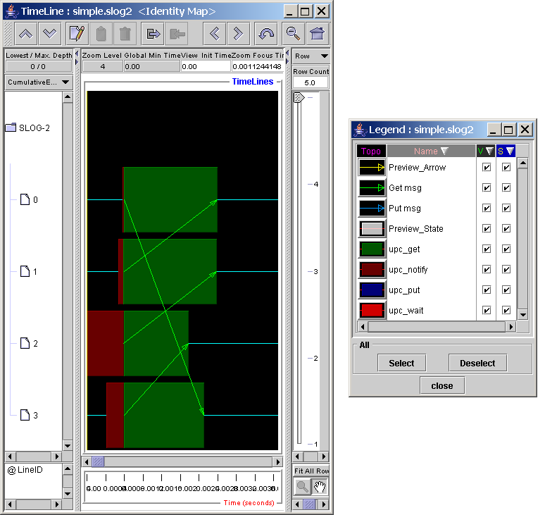
Once Jumpshot has finished loading the SLOG-2 file, you'll be presented with a window similar to the one shown in Figure 8.19.
Jumpshot gives you a timeline view of your program's trace file. A timeline view shows you the state of each node from a particular run at every point in time during the execution of your program. Each node from your run has a horizontal line drawn across the screen with boxes that tell you what operation that node was performing, and time increases as you travel towards the right of your screen. If you draw a perfectly straight vertical line at any point on the timeline, the line will intersect with every operation active at that particular instance of time. Because timeline views share many similarities with Gantt charts, they are often referred to as specialized Gantt charts.
For example, Figure 8.19 shows a trace file from a run with four threads. By examining the legend and the leftmost section of the timeline window, we see that each thread spends a different amount of time in the ‘upc_wait’ region (red boxes), which is a part of a barrier construct in UPC. Just after that, each node initiates a get operation from the thread above it, with thread 0 wrapping around to thread 3. Jumpshot denotes data transfers by drawing arrows from the data source, pointing to the destination of the data transfer operation.
As suggested above, this data example does not include function states, so we may interpret any black space (ie, the light blue lines) as time spent outside of UPC language operations, such as computation or OS system calls. If you convert a PPW trace file containing function information, you will see the states nested within each other. If your program has a deep nesting of function calls, this can become overwhelming very quickly.
For visualizing one-sided commmunication operations, PPW configures arrows for get and put operations to be drawn so that their direction shows the flow of data from one thread to the next. Put operations are drawn to suggest data is flowing from the initiating thread towards the passive remote thread, while get operations are drawn to suggest data is flowing from the remote thread where the data resides towards the initiating thread. For example, a get initiated on thread 0 for data residing on thread 3 will show an arrow originating on thread 3's timeline pointing towards the end of the get operation on thread 0.
To determine the time intervals for each one-sided operation, PPW configures the data transfer arrows to be drawn across the entire duration of the underlying get or put operation. This is a coarse approximation of the timing of the actual transfer; for technical reasons (DMA support in hardware that leaves the host CPU out of the loop, etc) it is generally not possible to accurately draw the exact start and end times of each data transfer.
Note: PPW does not display any nonblocking data transfers in any special way, so the timing of the arrows displayed for nonblocking get or put operations might be a little misleading as the data might not yet have finished transferring when the end of the arrow is drawn.
One good thing about Jumpshot is that it includes very good support for quickly browsing around a trace file by zooming and scrolling. This lets you easily jump around a very large trace file to quickly identify potential problem areas in your code.
To zoom in, make sure the magnifying glass icon is selected (the one above the ‘TimeLines’ blue text in the upper-right corner of the timeline window). Then, hold the left mouse button down on the part of the area you want to zoom in on, move the mouse to the rightmost side of the area you want to zoom in on, and release the mouse button (ie, highlight the area using the left mouse button).
To zoom out, use the button on the top of the screen that looks like a magnifying glass with a negative sign in it, or click on the button that looks like a house to reset the zoom and see the entire data file again.
You can use the scrollbar at the bottom of the screen to move through the data file. Alternatively, you can select the hand icon (next to the magnifying class, above the ‘TimeLines’ blue text in the upper-right corner of the timeline window) and scroll through the file using the same dragging motion you used before with the zoom operation.
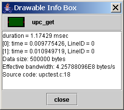
Right-clicking on any state box or arrow in the timeline display will bring up a dialog box similar to the one shown in Figure 8.20. PPW provides Jumpshot with source code information whenever possible when exporting data to SLOG-2, so using these popups is an excellent way to find out which line of code caused the operation you are viewing in Jumpshot. This is incredibly useful for spotting “communication leaks” in UPC programs, or for relating the performance data you're seeing back to parts of your original program.
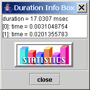
If you use the same dragging motion used in the zoom operation, but use your right mouse button instead of your left mouse button, you will get a popup as shown in Figure 8.21. Clicking on the statistics graphical button in the popup will bring up another window showing histrogram information for all active states in the selected region. This view is useful for viewing a summary of how time was spent in the region you just selected.
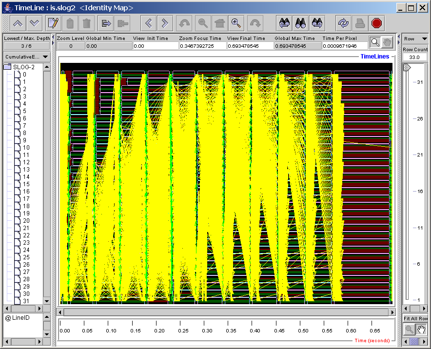
One of the more interesting aspects of Jumpshot deals with how it is able to display a large amount of trace data efficiently. Instead of drawing each individual box/arrow for a densely-populated region of time, Jumpshot instead displays preview states and preview arrows.
Preview states look just like a regular state box, except that they contain a histogram embedded inside them that describes the fraction of time taken by all of the state transitions encompassed by the region of time the preview state box encompasses. In other words, the preview state simply draws a histogram instead of drawing a bunch of individual boxes.
Preview arrows are similar to preview states, except that a single thick yellow arrow is used to represent a whole set of data transfers.
Figure 8.22 shows a trace file in which preview states and preview arrows are being displayed. This is the topmost view of a large trace view, and while the preview boxes and preview arrows are a little overwhelming, they are much easier to interpret than the jumble of colors that would result if each and every trace record were drawn instead of the preview objects that summarize multiple trace records.
Jumpshot provides several options to tweak how the histogram data is dislayed inside the preview boxes. The histogram calculation method can be changed by using the dropdown box above the node name list in the top left of the timeline window (ie, the box that says ‘CumulativeE...’). For more information on the available histogramming methods, refer to the Jumpshot user manual.
For more information about Jumpshot, refer to the online user manual which is available at http://www.mcs.anl.gov/perfvis or through the Jumpshot user interface by clicking on the green question button of the main Jumpshot window. The manual provided with Jumpshot can be very technical in some areas, but if you've skimmed through our brief introduction you should have an easier time of making sense of it.