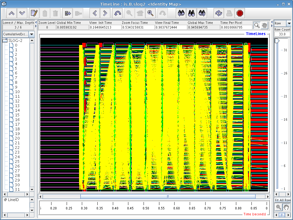
Figure 6.1: Jumpshot display of a 32-node IS benchmark run
Next: Summary, Previous: Generating Trace Data, Up: Top
After you start the Jumpshot viewer, and open up your new SLOG-2 file, you will be presented with a multitude of windows.
The main window in Jumpshot is the timeline window, which is shown in Figure 6.1. This window is the one that displays the timeline view we discussed before, and is where all the action happens when working with Jumpshot.
When opening a large trace file with Jumpshot, you will notice some interesting things being displayed. In Figure 6.1, we see a bunch of strange-looking boxes and arrows. These correspond to what Jumpshot calls “Preview drawables”; they are simply Jumpshot's way of summarizing a large amount of trace data for you. The summary boxes can be useful by themselves (very tiny histograms are drawn inside these boxes), but in general it is more useful to zoom in until you start noticing specific performance characteristics.
In our case with the IS benchmark, the overall screen doesn't really tell us much so we'll have to zoom in more closely to get an idea of what is going on. To zoom in, choose the magnifying glass tool from Jumpshot's toolbar and click on the screen, or select a horizontal section of the timeline by selecting it with your mouse (drag with the button down). Try to zoom in on one of the blocks with a bunch of yellow mush around it.
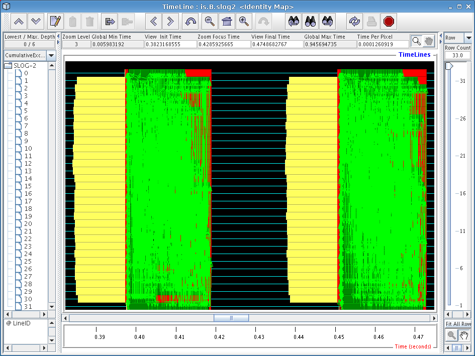
If you zoomed in on one of the blocks closer to the center of the screen, you should see a window similar to the one in Figure 6.2. This is starting to look a little more sane, since Jumpshot is now displaying real trace records instead of summary previews.
If you've never worked with timeline diagrams before, then you might be wondering what exactly Jumpshot is trying to tell you with this sort of display. Essentially, what Jumpshot does is draw one line per thread in your trace data file. On these lines, Jumpshot will draw boxes and arrows that represent states and communication from your run. Since we've decided to exclude function information in our trace file, we assume that anything drawn as black area can be attributed to “computation” (roughly speaking), and so any communication or other language-level operations will stick out on the timeline display.
Looking at Figure 6.2, we see two iterations of the IS sort benchmark kernel, which have similar behavior. One interesting thing we immediately notice is the big yellow boxes on the left side of the screen. Looking at the function key (not pictured), we find that these boxes correspond to calls to ‘upc_all_alloc’. As we found before in our profile data, the first and last threads in the system spend less time executing these functions. Since the function is a collective one, we can infer that these two threads were “late”, so we should look at the computational operations that immediately preceded these calls to figure out what is causing them to be slower than the other nodes.
One very useful tweak we've made to Jumpshot (by exploiting some interesting parts of its file format) is that by right-clicking on any particular box in the timeline window, a popup dialog will tell you exactly which line of code caused that particular operation. By right-clicking on one of the yellow boxes, we find that our old friend ‘upc_all_alloc’ on line 878 is definitely the perpetrator of this performance problem.
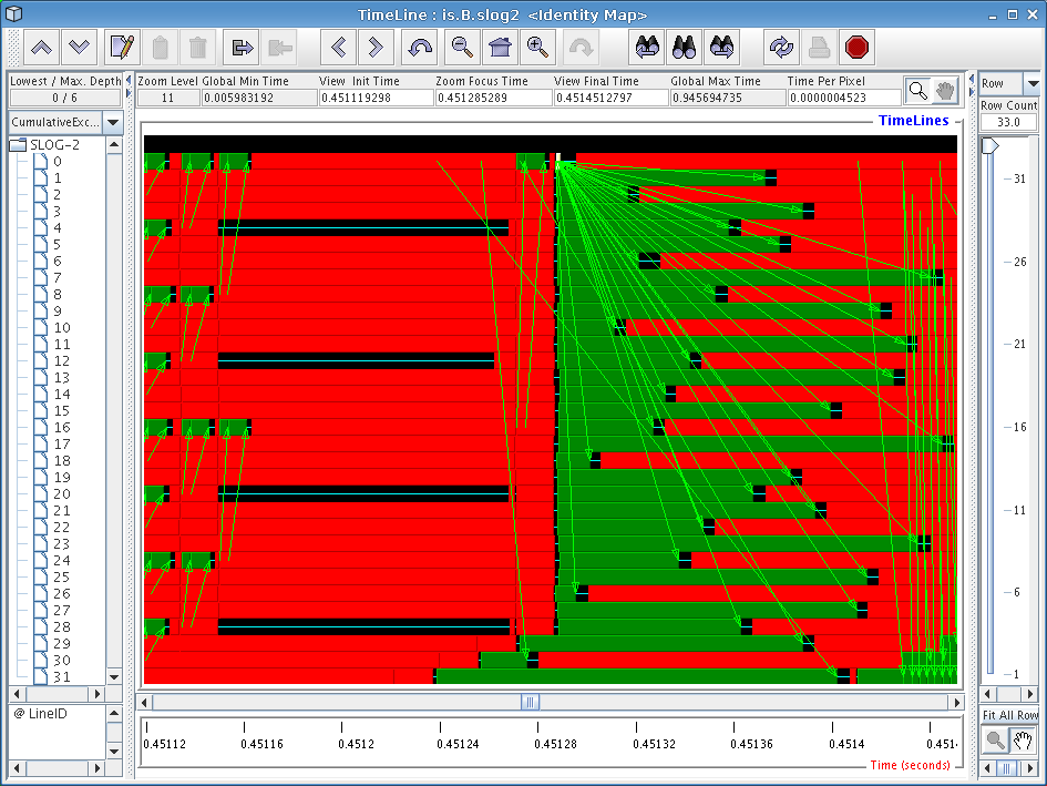
If you zoom in much closer by the red part of the trace file just to the right of the yellow ‘upc_all_alloc’ boxes, you will see a display similar to that in Figure 6.3. One thing that we immediately see here is a broadcast-style operation being implemented by using a string of ‘upc_memget’ operations. This particular benchmark was written before UPC had collective operations in its standard library, so rewriting the code to make use of these new collective operations might yield better performance.
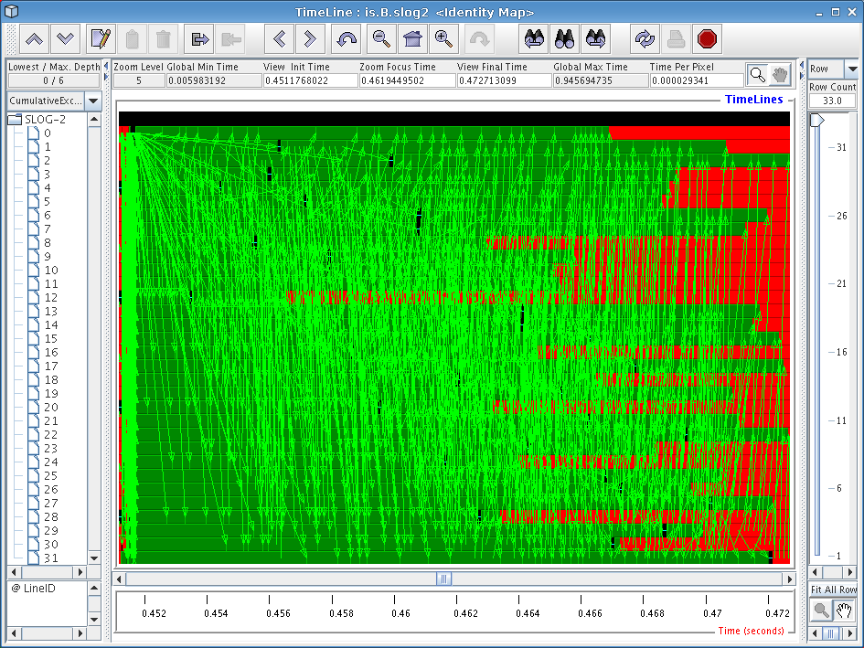
Scrolling over a little to the right of the previous broadcast operation and zooming out a little bit will produce a display similar to the one shown in Figure 6.4. Interestingly, this mass of communication stems from a single line of code, the ‘upc_memget’ operation on line 679 of is.c. Our profile data tells us that this single line of code takes up 30% of execution time in our runs, and this diagram provides visual cues as to why this might be the case: implementing an all-to-all communication operation on a Quadrics cluster as a sequence of unscheduled get operations does not yield very good overall performance. As with the previous broadcast, using the new collective functions would undoubtedly squeeze more performance out of our Quadrics cluster.
In this tutorial, we've only covered a few of Jumpshot's features. For more information on Jumpshot, refer to the frontend GUI reference chapter of the PPW user manual, or the Jumpshot user manual available from the Jumpshot website.