Figure 8.15: Load-balancing analysis
Next: Analysis Visualizations, Previous: Profile Charts, Up: Frontend GUI Reference
This section describes the analysis features offered by the PPW GUI, which can be accessed through the Analysis menu of the GUI.
PPW provides substantial application-level analysis functionality. The tool uses profile and/or trace data to automatically identify problem areas, or bottlenecks, within your application code. Application analysis is initiated by choosing Analysis > Run Application Analysis from the menu bar in the main PPW GUI. Choosing this menu option brings up a dialog for specifying various parameters to the application analysis process.
Within the Application Analysis dialog, the Do Filtering option specifies that high-level profile data should be used for filtering prior to the (potentially time-consuming) bottleneck identification steps. Choosing the Do Trace and Profile Analysis option indicates that both profile- and trace-based analysis should be performed. Trace-based analysis uses trace records to identify bottlenecks at a much greater level of detail, but also takes much longer and of course requires trace records to be present.
Another important option to be aware of is the Number of Analysis Threads. This specifies how many threads (units of execution on the computer running PPW) should be used to perform the analysis processing. This value is important for optimizing the performance of the analysis process. The field will be filled in with a guess of how many “processors” (or cores) your machine has. This should be a reasonable number of analysis threads to use, but you may want to adjust the value based on specific knowledge of your system. For example, if you know your system actually has more processors or otherwise supports more parallel units of execution, increasing the number of analysis threads may improve performance. Similarly, if you know you actually have fewer processors available, or will be utilizing CPU resources for other applications, decreasing the number of analysis threads may be advisable.
Click Run to start the analysis process. A dialog will appear with a progress bar indicating the status of the processing. Once the process is complete, analysis visualizations will become available within the PPW GUI.
Scalability analysis is initiated by choosing Analysis > Run Scalability Analysis from the menu bar in the main PPW GUI. There are currently no parameters to the scalability analysis processing, so the analysis should begin immediately. After it completes, scalability-related analysis visualizations will become available within the PPW interface.
Memory leak analysis is initiated by choosing Analysis > Run Memory Leak Analysis from the menu bar in the main PPW GUI. For UPC programs the analysis should begin. After it completes, memory leak analysis visualizations will become available within the PPW interface.
After one or more analyses have been run, the resulting analysis data can be saved to the currently opened PAR file using the Analysis > Save analysis data to current PAR file option in PPW's menu bar. Alternatively, a new PAR file containing the analysis data can be saved by choosing the Analysis > Save new PAR file with analysis data... option. This will bring up a dialog allowing you to specify the name and location of the file to save.
The load-balancing analysis is accessed by choosing Analysis > Other Analyses > Load-balancing analysis from the menu bar in the main PPW GUI. Choosing this menu option brings up a dialog that describes this analysis. By clicking the ‘Next’ button, PPW will analyze the profile data for the currently-open file. After a short delay, the dialog will change to show you a list of lines of code with a load-balancing problem.
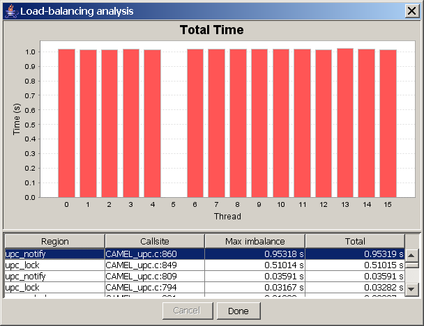
See Figure 8.15 for an example of how the interface looks after running the load-balancing analysis.
Clicking on each of the entries in the list below will change the graph in the top half of the screen, showing you the breakdown of time spent on that particular line of code across all nodes on which the program was run.
The load-balancing analysis uses a very simple method for detecting load-balancing problems across your application. The analysis uses the heuristic that the sum of time spent executing each line of profiled code (such as calls to UPC library functions, or lines of code incurring communication in UPC) should take roughly the same amount of time on each node in the system. The analysis examines profile data for each profiled line of code, and flags any line of code where one node's time differs by more than 25 percent than the average time taken by all the nodes. After the analysis is finished running, it displays all flagged source lines, sorted by the greatest difference of time from the average (the ‘Max imbalance’ column) and shows the sum of differences of each node from the mean in the ‘Total’ column.
In the example screenshot above, line number 860 of CAMEL_upc.c had a max imbalance of 0.95 seconds, meaning that one node's sum of execution time for line 860 differed from the mean time across all nodes by 0.95 seconds. By examining the top of the screen we see that node five is the culprit. The ‘upc_notify’ line in this example belongs to a barrier synchronization construct; thus, the graph tells us that most nodes end up waiting in a barrier for node five to catch up to them. This clearly shows the example program has load-balancing problems (node five is a slowpoke!), and that by fixing the imbalance on line 860, we could increase this example application's efficiency.
The load-balancing analysis can be even more useful when combined with program phase information recorded using the measurement API described later in the manual. For details on how to use PPW's measurement API to record application-specific performance information, see API Reference.